Estimating Forcing Functions for the FitzHugh-Nagumo Equations
This page provides a demonstration of the use of forcing functiona perturbed set of FitzHugh-Nagumo Equations:


Here we will assume knowledge of $a$, $b$ and $c$, and estimate $g(t)$ from data.
The format of this demonstration follows that detailed in FhNEx.html and commentary will therefore be restricted to terms unique to forcing function estimation.
Contents
- RHS Functions
- Observation times
- Various Parameters
- Extra Information for the System:
- Penalties on Forcing Functions
- Initial Forcing Estimates
- Create trajectories
- Set up observations
- Fitting parameters
- Optimisation control
- Setting up functional data objects
- Smooth the data
- Re-Smooth with a Model-Based Penalty
- Now do the profiled estimation
- Examine Forcing Functions
- Calculate a Sample Information Matrix
- Calculate Hotelling Distance from Zero
RHS Functions
Since we are using a linear function to begin with, we make use of the forcing set of functions (although fhnfunodep will be used to produce data).
addpath('../FhN')

odefn       = @fhnfunodep;        % Function for ODE solver (exact)

fn.fn       = @forcingfun;        % RHS function

fn.dfdx     = @forcingdfdx;       % Derivative wrt inputs (Jacobian)
fn.dfdp     = @forcingdfdp;       % Derviative wrt parameters

fn.d2fdx2   = @forcingd2fdx2;     % Hessian wrt inputs
fn.d2fdxdp  = @forcingd2fdxdp;    % Cross derivatives wrt inputs and parameters
fn.d2fdp2   = @forcingd2fdp2;     % Hessian wrt parameters

fn.d3fdx2dp = @forcingd3fdx2dp;   % Third derivative wrt inputs, inputs, pars
fn.d3fdx3   = @forcingd3fdx3;     % Third derivative wrt inputs
fn.d3fdxdp2 = @forcingd3fdxdp2;   % Third derivative wrt inputs, pars and pars
Warning: Name is nonexistent or not a directory: ..\FhN.
Observation times
tspan = 0:0.05:20;    % Observation times

obs_pts{1} = 1:length(tspan);      % Which components are observed at
obs_pts{2} = 1:length(tspan);      % which observation times.

tfine = 0:0.05:20;    % Times to plot solutions
Various Parameters
y0 = [-1,1];               % Initial conditions
pars0 = [0.2; 0.2; 3];     % Parameters for the FitzHugh-Nagumo equations

% Set up a perturbation functional data object

basis_obj = create_bspline_basis([0 20],42,3,0:0.5:20);
quadvals = MakeQuadPoints(0:0.5:20,21);      % We will need to use
basis_obj = putquadvals(basis_obj,quadvals); % quadrature points later

%pcoef = zeros(42,1);
pcoef(floor(42/3):(ceil(42/3)+5)) = 10;
fd_obj = fd(pcoef,basis_obj);

% Finally decide on a noise level:

sigma = 0.25;              % Noise Level
Extra Information for the System:
In particular, we need to specify the original ODEs and their derifatives with respect to components (in this case the FitzHugh-Nagumo Equations) and also the option of adding further information for the original system.
fn_extras.fn      = @fhnfun;    % Original function
fn_extras.dfdx    = @fhndfdx;   % First derivative
fn_extras.d2fdx2  = @fhnd2fdx2; % Second derivative
fn_extras.d3fdx3  = @fhnd3fdx3; % Third derivative

fn_extras.extras  = [];        % Original information to fn_extras.fn.

% We also need to add parameters:

fn_extras.pars = pars0;

% We also need to specify a basis for the forcing components and a vector
% indicating which components are to be forced.

fn_extras.basisp = {basis_obj};   % Cell array of basis functions.
fn_extras.which  = 1;             % Force the first component of the
                                  % system only.

% Note that although we are only forcing one component here, the forcing
% basis is still represented as a cell array and we could equally have
% estimated a number of forcing functions.
Penalties on Forcing Functions
We can also place roughness penalties on forcing functions, these will then occur as inputs into Profile_GausNewt.
pen   = @forcingpen;   % Penalty
dpen  = @forcingdpen;  % Derivative with respect to forcing co-efficients
d2pen = @forcingd2pen; % Second derivative

% These penalty functions also require extra arguments in the form of a
% struct to specify the basis, the degree of smoothing and the smoothing
% penalty:

pen_extras. basis = {basis_obj}; % Same basis as fn_extras.
pen_extras.deg    = 2;           % Penalize the second derivative
pen_extras.lambda = 0.0001;      % Smoothing parameter.
Initial Forcing Estimates
We start off assuming the forcing function is zero. Since the coefficients of a basis expansion for it occur as parameters in the profiled estimation scheme we set them as:
startpars = zeros(getnbasis(basis_obj),1);
Create trajectories
odeopts = odeset('RelTol',1e-13);
[full_time,full_path] = ode45(odefn,tspan,y0,odeopts,pars0,fd_obj);
[plot_time,plot_path] = ode45(odefn,tfine,y0,odeopts,pars0,fd_obj);
Set up observations
Tcell = cell(1,size(full_path,2));
path = Tcell;

for i = 1:length(obs_pts)
    Tcell{i} = full_time(obs_pts{i});
    path{i} = full_path(obs_pts{i},i);
end

% add noise

Ycell = path;
for i = 1:length(path)
    Ycell{i} = path{i} + sigma*randn(size(path{i}));
end

% and set wts

wts = [];

if isempty(wts)                             % estimate wts if not given
    for i = 1:length(Ycell)
        wts(i) = 1./sqrt(var(Ycell{i}));
    end
end
Fitting parameters
lambda = 1000;          % Smoothing for model-based penalty
lambda = lambda*wts;

lambda0 = 1;   % Smoothing for 1st-derivative penalty

nknots = 401;    % Number of knots to use.
nquad = 5;       % No. between-knots quadrature points.
norder = 6;      % Order of B-spline approximation
Optimisation control
lsopts_out = optimset('DerivativeCheck','off','Jacobian','on',...
    'Display','iter','MaxIter',1000,'TolFun',1e-8,'TolX',1e-10);

% Other observed optimiation control
lsopts_other = optimset('DerivativeCheck','off','Jacobian','on',...
    'Display','on','MaxIter',1000,'TolFun',1e-14,'TolX',1e-14,...
    'JacobMult',@SparseJMfun);

% Optimiation control within profiling
lsopts_in = optimset('DerivativeCheck','off','Jacobian','on',...
    'Display','off','MaxIter',1000,'TolFun',1e-14,'TolX',1e-14,...
    'JacobMult',@SparseJMfun);
Setting up functional data objects
% set up knots

range = [min(full_time),max(full_time)];  % range of observations

knots_cell = cell(size(path));            % knots for each basis
knots_cell(:) = {linspace(range(1),range(2),nknots)};

% set up bases

basis_cell = cell(1,length(path));   % Create cell arrays.
Lfd_cell = cell(1,length(path));

nbasis = zeros(length(path),1);

bigknots = knots_cell{1};            % bigknots used for quadrature points
nbasis(1) = length(knots_cell{1}) + norder - 2;
for i = 2:length(path)
    bigknots = [bigknots knots_cell{i}];
    nbasis(i) = length(knots_cell{i}) + norder -2;
end

quadvals = MakeQuadPoints(bigknots,nquad);   % Create simpson's rule
                                             % quadrature points and values
for i = 1:length(path)
    basis_cell{i} = MakeBasis(range,nbasis(i),norder,...  % create bases
        knots_cell{i},quadvals,4);                        % with quadrature
    Lfd_cell{i} = fdPar(basis_cell{i},1,lambda0);         % pts  attatched
end
Smooth the data
DEfd = smoothfd_cell(Ycell,Tcell,Lfd_cell);
coefs = getcellcoefs(DEfd);

devals = eval_fdcell(tfine,DEfd,0);
for i = 1:length(path)
    subplot(length(path),1,i);
    plot(plot_time,plot_path(:,i),'b','LineWidth',2);
    hold on;
    plot(tfine,devals{i},'r','LineWidth',2);
    plot(Tcell{i},Ycell{i},'b.');
    hold off;
end

Re-Smooth with a Model-Based Penalty
[newcoefs,resnorm2] = lsqnonlin(@SplineCoefErr,coefs,[],[],...
    lsopts_other,basis_cell,Ycell,Tcell,wts,lambda,fn,[],startpars,...
    fn_extras);

tDEfd = Make_fdcell(newcoefs,basis_cell);

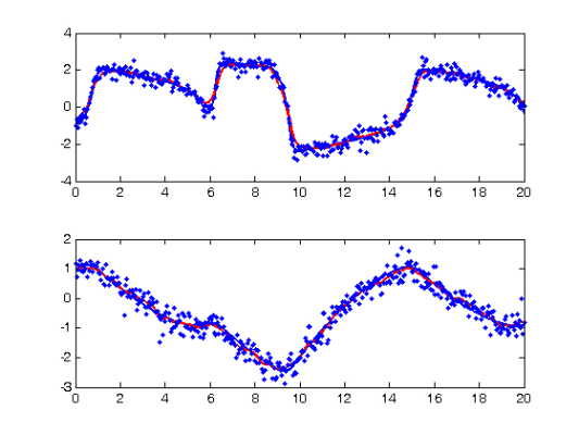
% plot results along with exact solution, there is a noticeable lack of
% fit.

devals = eval_fdcell(tfine,tDEfd,0);
for i = 1:length(Ycell)
    subplot(length(Ycell),1,i);
    plot(tfine,devals{i},'r','LineWidth',2);
    hold on;
    plot(Tcell{i},Ycell{i},'b.');
    plot(plot_time,plot_path(:,i),'c');
    hold off
end
Optimization terminated: relative function value
 changing by less than OPTIONS.TolFun.

Now do the profiled estimation
Recall that at this point we are estimating the coefficients of the forcing functions.
[fcoefs,DEfd] = Profile_GausNewt(startpars,lsopts_out,tDEfd,fn,lambda,...
    Ycell,Tcell,wts,[],lsopts_in,fn_extras,pen,dpen,pen_extras);

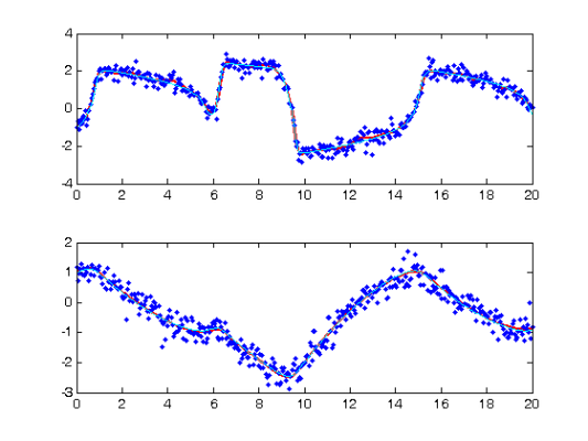
% DEfd now takes the form of a smooth to the data and we can see that it
% fits better:

devals = eval_fdcell(tfine,DEfd,0);
for i = 1:length(path)
    subplot(length(path),1,i);
    plot(tfine,devals{i},'r','LineWidth',2);
    hold on;
    plot(Tcell{i},Ycell{i},'b.');
    plot(plot_time,plot_path(:,i),'c');
    hold off
end
 Iteration       steps    Residual   Improvement   Grad-norm     parameters
     1           1         126.093      0.592753        0.298     -0.74061   -0.066343     0.51962     -1.4236    -0.72229     0.45195    0.056012     -1.0448     0.36335     -0.3683     -1.0082   -0.005413    -0.95034      8.7874     -2.6424      1.3379      3.5346       4.958      7.9916       -1.69      8.9789      7.6286     -1.8416     0.67843    -0.45554      2.3315   -0.092889     0.31005     -1.0432      2.4937     -2.8465     -3.2763     0.12289    -0.53359     0.72481    -0.97313     0.92401     -1.2589     0.73558    -0.62486     0.36293      1.9134
     2           1         72.7815      0.422797       0.0348     -0.543809    0.0390957     0.516403       -1.356    -0.665423     0.432098    0.0144772    -0.977691     0.377309     0.243895    -0.780672      1.15339     -1.13211      16.0818      3.05923    -0.152166      7.74569      12.3853      8.40364      -1.6618      6.87211      8.87325     0.309595    -0.575085    -0.684515      2.02412    0.0723844     0.403837     0.293083    0.0533429    -0.438236    -0.782215     -1.51268    0.0342214     0.695885    -0.924587     0.921273     -1.23676     0.664204    -0.593956     0.414861      1.71205
     3           1         47.4938      0.347447       0.0049     -0.715957   -0.0300497     0.561359      -1.2115    -0.506859     0.649419     0.283191    -0.797805     0.712243      0.44896    -0.389681     0.148751      0.38651      7.89654      11.4206      1.92934      8.62524      13.0305      8.78573   -0.0574364      2.13521      7.14525     0.191142      -1.6327     -1.39984      1.74743    -0.185594     0.348316    -0.217555     0.515205    -0.157832     0.173842     -1.05544    -0.221741     0.693638     -0.91932     0.913194     -1.20305     0.713828    -0.588338     0.367317      1.68152
     4           1         42.5592        0.1039     0.000321     -0.715045    -0.041507     0.563264     -1.19524    -0.484007     0.671902     0.311927    -0.689212     0.751827     0.615595    -0.473893     0.459882   -0.0831338      9.12517      12.3077      6.32168      9.84922      12.3152      8.96157     0.683865    -0.820837      2.59282   -0.0508123     -1.09665      -1.1372      1.88296   -0.0315437     0.394611    -0.220598     0.354213    -0.259916     0.379593    -0.841356    -0.237914     0.757766    -0.922057     0.938468      -1.2212     0.690566       -0.606     0.374637      1.69128
     5           1         42.3398    0.00515544    3.84e-005     -0.720761   -0.0416537     0.563535     -1.19708    -0.486534     0.669067     0.306695    -0.693857     0.746413     0.610066    -0.469159     0.440291   -0.0508425      9.05762      12.2901      7.48831      10.2603      12.2103      8.90905     0.826736     -1.32213      0.85847    -0.422614    -0.928106     -1.19913      1.90477   -0.0708986     0.407958    -0.241958     0.357149    -0.256231     0.369341    -0.817005    -0.241774     0.753444    -0.916983      0.93269     -1.21777     0.690004    -0.604909     0.372529      1.69073
     6           1          42.339  1.89533e-005    5.64e-006     -0.720825    -0.041736     0.563424     -1.19735    -0.486874     0.668637     0.306201    -0.694535     0.746017     0.609175    -0.469827     0.440023   -0.0504314      9.05743       12.303      7.56272      10.2486      12.2188      8.90285     0.834049     -1.33174     0.732646    -0.458082     -0.90851     -1.20296      1.90775   -0.0738449     0.408676    -0.240962     0.357092     -0.25465       0.3566    -0.814203    -0.242588     0.754458     -0.91737     0.933962     -1.21846     0.689439    -0.604891     0.373614      1.69102
     7           1          42.339  1.45619e-008    1.38e-007     -0.720822   -0.0417374     0.563415     -1.19735    -0.486883     0.668626     0.306195    -0.694572     0.746036     0.609076    -0.469778     0.439908   -0.0502118       9.0568      12.3036      7.56565      10.2476      12.2187      8.90246     0.834309     -1.33185     0.729867    -0.458573    -0.907431      -1.2033      1.90798   -0.0741554     0.408809    -0.241104     0.357339    -0.254891     0.356914    -0.814291    -0.242613     0.754476    -0.917333      0.93397     -1.21846     0.689354    -0.604886     0.373709      1.69101
     8           1          42.339  1.26056e-010    5.35e-009     -0.720822   -0.0417377     0.563414     -1.19735    -0.486883     0.668625     0.306194    -0.694573     0.746036     0.609071    -0.469779     0.439909   -0.0502163      9.05682      12.3036      7.56575      10.2475      12.2187      8.90245     0.834316     -1.33185     0.729817    -0.458599    -0.907401     -1.20329      1.90798   -0.0741527     0.408801    -0.241093     0.357339    -0.254889     0.356877    -0.814287    -0.242609     0.754477    -0.917329     0.933971     -1.21846     0.689348    -0.604886     0.373714      1.69101

Examine Forcing Functions
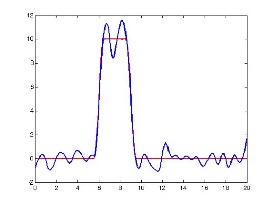
First we constitute the approximated forcing function:
fd_approx = fd(fcoefs,basis_obj);

% Now plot the results along with the original forcing function:

force_devals = eval_fd(tfine,fd_obj);
approx_devals = eval_fd(tfine,fd_approx);

subplot(1,1,1)
plot(tfine,force_devals,'r','LineWidth',2);
hold on
plot(tfine,approx_devals,'b','LineWidth',2);
hold off

Calculate a Sample Information Matrix
d2Jdp2 = make_d2jdp2(DEfd,fn,Ycell,Tcell,lambda,fcoefs,[],wts,...
    fn_extras,d2pen,pen_extras);

d2JdpdY = make_d2jdpdy(DEfd,fn,Ycell,Tcell,lambda,fcoefs,[],wts,fn_extras);

dpdY = -d2Jdp2\d2JdpdY;

S = make_sigma(DEfd,Tcell,Ycell,0);

Cov = dpdY*S*dpdY';
Calculate Hotelling Distance from Zero
Look at the distance of fcoefd from 0 with respect to the metric defined by Cov. This is a heuristic Wald test for the goodness of fit of the original equations.
disp(['Goodness of fit = ',num2str(fcoefs'*inv(Cov)*fcoefs)])
Goodness of fit = 1800.802