Profile Estimation Experiments

Contents

RHS Functions

odefn       = @rossfunode;    % Function for ODE solver

fn.fn       = @rossfun;       % RHS function
fn.dfdx     = @rossdfdx;      % Derivative wrt inputs
fn.dfdp     = @rossdfdp;      % Derviative wrt parameters

fn.d2fdx2   = @rossd2fdx2;    % Hessian wrt inputs
fn.d2fdxdp  = @rossd2fdxdp;   % Hessian wrt inputs and parameters
fn.d2fdp2   = @rossd2fdp2;    % Hessian wrt parameters.

fn.d3fdx3   = @rossd3fdx3;    % Third derivative wrt inputs.
fn.d3fdx2dp = @rossd3fdx2dp;  % Third derivative wrt intputs, inputs and pars.
fn.d3fdxdp2 = @rossd3fdxdp2;  % Third derivative wrt inputs, pars and pars.

Observation times

tspan = 0:0.05:20;    % Observation times
tfine = 0:0.05:20;    % Times to plot solutions

 obs_pts = {1:401,   1:401, 1:401;    % Rows represent replications
            1:2:401, 1:201, 201:401};

y0 = [1.13293; -1.74953; 0.02207];  % Initial conditions
y0 = repmat(y0',2,1);

parind = 1:3;
parind = repmat(parind,size(y0,1),1);

Other parameters

pars = [0.2; 0.2; 3];           % Parameters

sigma = 0.5;                    % Noise Level
%sigma = 0;

%jitter = 0;                     % Perturbation for starting parameters
jitter = 0.2;

Fitting parameters

lambdas = 1000;                   % Smoothing for model-based penalty

lambda0 = 1;   % Smoothing for 1st-derivative penalty

wts = [];         % Loading factor for each component (empty means use
% wts = [1 0];    % inverse of standard error).

nknots = 401;    % Number of knots to use.

nquad = 5;       % No. between-knots quadrature points.
norder = 3;      % Order of B-spline approximation

Profiling optimisation control

maxit1 = 100;      % Maximum iterations interior of profiling
maxit0 = 100;     % Maximum iterations for outer optimization

lsopts_out = optimset('DerivativeCheck','off','Jacobian','on',...
    'Display','iter','MaxIter',maxit0,'TolFun',1e-8,'TolX',1e-10);

% Other observed optimiation control
lsopts_other = optimset('DerivativeCheck','off','Jacobian','on',...
    'Display','off','MaxIter',maxit0,'TolFun',1e-14,'TolX',1e-14,...
    'JacobMult',@SparseJMfun);

% Optimiation control within profiling
lsopts_in = optimset('DerivativeCheck','off','Jacobian','on',...
    'Display','off','MaxIter',maxit1,'TolFun',1e-14,'TolX',1e-14,...
    'JacobMult',@SparseJMfun);

First create a trajectory

odeopts = odeset('RelTol',1e-13);

for i = 1:size(y0,1)
    [full_time(:,i),full_path(:,:,i)] = ode45(odefn,tspan,y0(i,:),odeopts,pars);
    [plot_time(:,i),plot_path(:,:,i)] = ode45(odefn,tfine,y0(i,:),odeopts,pars);
end
% set up observations

Tcell = cell(size(y0));
path = cell(size(y0));

for i = 1:size(obs_pts,1)
    for j = 1:size(obs_pts,2)
        Tcell{i,j} = full_time(obs_pts{i,j},i);
        path{i,j} = full_path(obs_pts{i,j},j,i);
    end
end

% add noise

Ycell = path;
for i = 1:size(path,1)
    for j = 1:size(path,2)
        Ycell{i,j} = path{i,j} + sigma*randn(size(path{i,j}));
    end
end

Setting up functional data objects

% set up knots

range = zeros(2,2);              % Range of observations
knots_cell = cell(size(path));   % Knots for each basis

for i = 1:size(path,1)
    range(i,:) = [min(full_time(:,i)),max(full_time(:,i))];
    knots_cell(i,:) = {linspace(range(i,1),range(i,2),nknots)};
end

% set up bases

basis_cell = cell(size(path));      % Create cell arrays.
Lfd_cell = cell(size(path));

nbasis = zeros(size(path));

bigknots = cell(size(path,1),1);    % bigknots used for quadrature points
bigknots(:) = {[]};
quadvals = bigknots;

for i = 1:size(path,1)
    for j = 1:size(path,2)
        bigknots{i} = [bigknots{i} knots_cell{i,j}];
        nbasis(i,j) = length(knots_cell{i,j}) + norder -2;
    end
    quadvals{i} = MakeQuadPoints(bigknots{i},nquad);
end

for i = 1:size(path,1)        % create bases and quadrature points
    for j = 1:size(path,2)
        basis_cell{i,j} = MakeBasis(range(i,:),nbasis(i,j),norder,...
            knots_cell{i,j},quadvals{i},1);
        Lfd_cell{i,j} = fdPar(basis_cell{i,j},1,lambda0);
    end
end

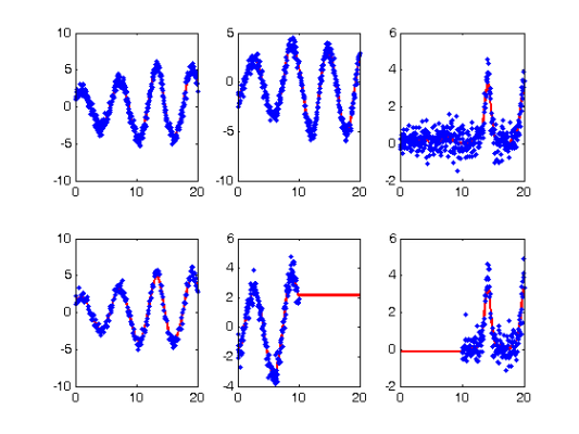
Smooth the data

DEfd = smoothfd_cell(Ycell,Tcell,Lfd_cell);
coefs = getcellcoefs(DEfd);

devals = eval_fdcell(tfine,DEfd,0);
for i = 1:size(path,1)
    for j = 1:size(path,2)
        subplot(size(path,1),size(path,2),(i-1)*size(path,2)+j)
        plot(tfine,devals{i,j},'r','LineWidth',2);
        hold on;
        plot(Tcell{i,j},Ycell{i,j},'b.');
        hold off;
    end
end



% Jitter parameters
startpars = pars + jitter*randn(length(pars),1);
disp(startpars)

    0.5512
   -0.0758
    2.7100

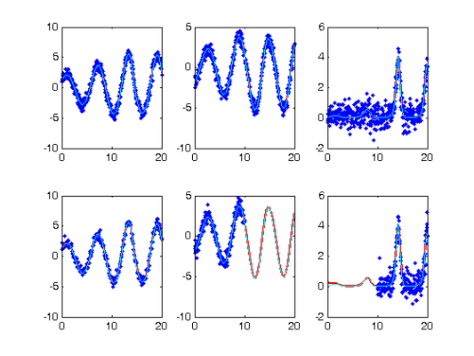
Re-smoothing with model-based penalty

lambda = lambdas*ones(size(Ycell)); % vectorize lambda

if  isempty(wts)                    % estimate wts if not given
    wts = zeros(size(path));
    for i = 1:numel(Ycell)
        if  ~isempty(Ycell{i})
            wts(i) = 1./sqrt(var(Ycell{i}));
        end
    end
end

% Call the Gauss-Newton solver

[newcoefs,resnorm2] = lsqnonlin(@SplineCoefErr_rep,coefs,[],[],...
    lsopts_other,basis_cell,Ycell,Tcell,wts,lambda,fn,[],startpars,parind);

tDEfd = Make_fdcell(newcoefs,basis_cell);

% Plot results along with exact solution

devals = eval_fdcell(tfine,tDEfd,0);
for i = 1:size(path,1)
    for j = 1:size(path,2)
        subplot(size(path,1),size(path,2),(i-1)*size(path,2)+j)
        plot(tfine,devals{i,j},'r','LineWidth',2);
        hold on;
        plot(Tcell{i,j},Ycell{i,j},'b.');
        plot(plot_time,plot_path(:,j,i),'c');
        hold off
    end
end

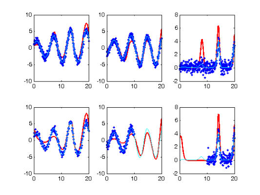
Perform the Profiled Estimation

[newpars,newDEfd_cell] = Profile_GausNewt_rep(startpars,lsopts_out,parind,...
    DEfd,fn,lambda,Ycell,Tcell,wts,[],lsopts_in);

disp(newpars);

 Iteration       steps    Residual   Improvement   Grad-norm     parameters
     1           1         705.665      0.439788          415     0.11709     0.56071      2.6582
     2           1         265.567      0.623664          129     0.22341     0.21112      2.7689
     3           1         246.678     0.0711267         8.13     0.19652     0.19984      2.9816
     4           1           246.6     0.0003149       0.0127     0.19834     0.19658       2.981
     5           1           246.6  2.55662e-007      0.00201     0.19832     0.19627      2.9803
     6           1           246.6  1.07281e-009     0.000135     0.19832     0.19625      2.9802
    0.1983
    0.1963
    2.9802

Plot Smooth with Profile-Estimated Parameters

devals = eval_fdcell(tfine,newDEfd_cell,0);
for i = 1:size(path,1)
    for j = 1:size(path,2)
        subplot(size(path,1),size(path,2),(i-1)*size(path,2)+j)
        plot(tfine,devals{i,j},'r','LineWidth',2);
        hold on;
        plot(Tcell{i,j},Ycell{i,j},'b.');
        plot(plot_time,plot_path(:,j,i),'c');
        hold off
    end
end

Comparison with Smooth Using True Parameters

coefs = getcellcoefs(DEfd);

[truecoefs,resnorm4] = lsqnonlin(@SplineCoefErr_rep,coefs,[],[],...
    lsopts_other,basis_cell,Ycell,Tcell,wts,lambda,fn,[],pars,parind);

trueDEfd_cell = Make_fdcell(truecoefs,basis_cell);

devals = eval_fdcell(tfine,trueDEfd_cell,0);
for i = 1:size(path,1)
    for j = 1:size(path,2)
        subplot(size(path,1),size(path,2),(i-1)*size(path,2)+j)
        plot(tfine,devals{i,j},'r','LineWidth',2);
        hold on;
        plot(Tcell{i,j},Ycell{i,j},'b.');
        plot(plot_time,plot_path(:,j,i),'c');
        hold off
    end
end

Squared Error Performance

newpreds = eval_fdcell(Tcell,newDEfd_cell,0);
new_err = cell(size(newpreds));
for i = 1:numel(path)
    if  ~isempty(newpreds{i})
        new_err{i} = wts(i)*(newpreds{i} - Ycell{i}).^2;
    end
end

new_err = mean(cell2mat(reshape(new_err,numel(new_err),1)));

truepreds = eval_fdcell(Tcell,trueDEfd_cell,0);
true_err = cell(size(truepreds));
for i = 1:numel(path)
    if  ~isempty(truepreds{i})
        true_err{i} = wts(i)*(truepreds{i} - Ycell{i}).^2;
    end
end

true_err = mean(cell2mat(reshape(true_err,numel(true_err),1)));

disp([new_err true_err]);

    0.1365    0.1366

Calculate a Sample Information Matrix

d2Jdp2 = make_d2jdp2_rep(newDEfd_cell,fn,Ycell,Tcell,lambda,newpars,...
    parind,[],wts);

d2JdpdY = make_d2jdpdy_rep(newDEfd_cell,fn,Ycell,Tcell,lambda,newpars,...
    parind,[],wts);

dpdY = -d2Jdp2\d2JdpdY;

S = make_sigma(DEfd,Tcell,Ycell,0);

Cov = dpdY*S*dpdY';

%  Standard errors

StdDev = sqrt(diag(Cov));

%  Correlations

Corr = Cov./(StdDev*StdDev');

%  Display these results

disp('Approximate covariance matrix for parameters:')
disp(num2str(Cov))

disp('Approximate standard errors of parameters:')
disp(num2str(StdDev'))

disp('Approximate correlation matrix for parameters:')
disp(num2str(Corr))

Approximate covariance matrix for parameters:
9.1968e-006  3.408e-005  0.00010678
 3.408e-005  0.00024914   0.0007058
 0.00010678   0.0007058   0.0026202
Approximate standard errors of parameters:
0.0030326    0.015784    0.051188
Approximate correlation matrix for parameters:
      1     0.71197     0.68786
0.71197           1     0.87355
0.68786     0.87355           1

Published with MATLAB® 7.1